
I build robots that know where they are.
- Each dot is a guess at where the robot is.
- Its four sensors measure the walls. Guesses that don’t match fade away.
- The guesses agree. Now it knows where it is.
Rendered in Blender from VEX’s field model, running the robot’s own code.
I’m Howard Wang, a high school student who builds and programs robots.
- Wheels alone
- 0.0 in off
- With sensors
- searching
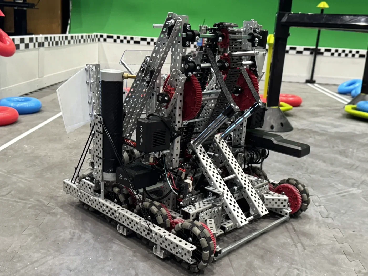
Our VEX robot
Team 1658S, 2025–26
For the first part of every match the robot drives itself, with nobody at the controls. I write the code that tells it where it is on the field.

An autonomous run, from above
- The robot drives a route on its own. The gray trail is where its wheels think it went.
- A bump knocks the wheels 15 inches off. The sensors still put the robot in the right place.
Rendered in Blender on VEX’s field model, running the robot’s own code. The bump is simulated.
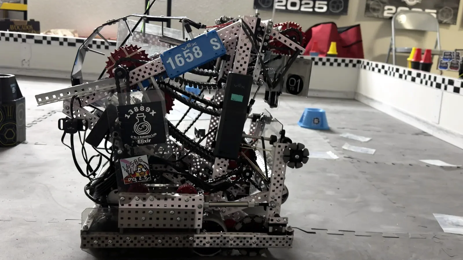
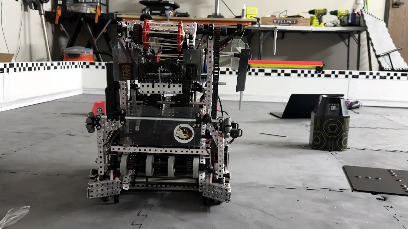
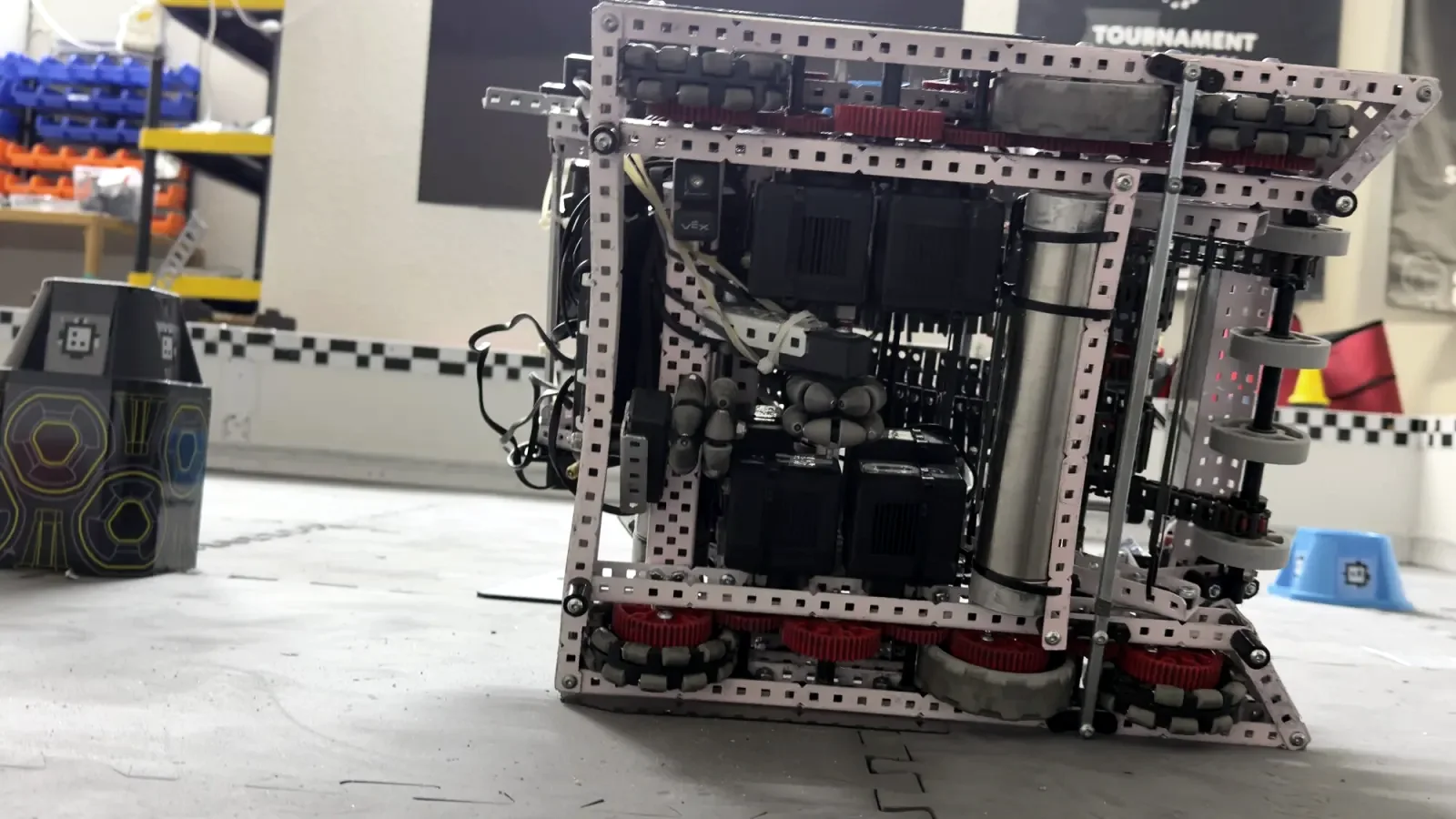
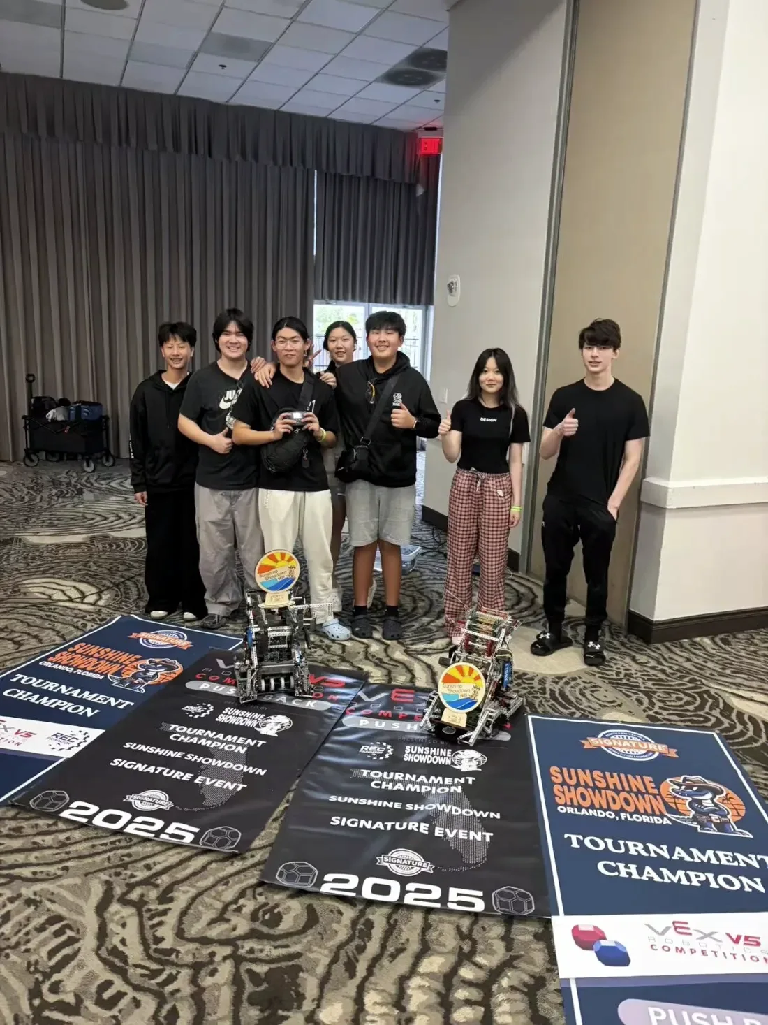
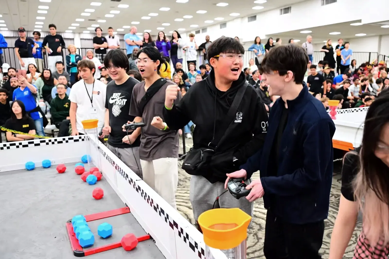
Tournament champions at two Signature Events
Push Back season, Sunshine Showdown, Orlando, 2025
A team of five, and two Signature Event wins in one season.
Engineering notes for this chapter
I’m building a stack that gives the robot a better-grounded estimate. A Monte Carlo localization filter with 450 particles recovers absolute position from four distance sensors. An extended Kalman filter fuses that with odometry, so motion stays smooth without trusting bad measurements. A chi-square gate, outlier rejection and rate-limited corrections keep one bad reading from yanking the motion controller. The opening film, Fig. 1 and Fig. 2 all show this filter at work.
The prototype compares the fused position with odometry-only runs over repeated autonomous paths, with contact and wheel slip. Next I plan to publish the implementation, the test method and the logs, so other VEX teams can reproduce the result or find where it breaks.
1if (!turnCorrectionSuppressed && !sensorsStale &&
2    correctionGeometryReady && correctionStable &&
3    correctionCloseToTrack &&
4    (threeSensorCorrectionReady || twoSensorCorrectionReady)) {
5  const float nisGate = threeSensorCorrectionReady
6      ? config.fusion.nisGate
7      : config.fusion.nisGate * kTwoSensorCorrectionNisScale;
8  if (nis <= nisGate) {
9    ekf.update(rawMeas.pose, rawMeas.covariance);
10    correctionAccepted = true;
11  }
12}localization.cpp: a fix reaches the Kalman filter only if every check passes, including an innovation gate of 8.0.A humanoid robot
Summer internship, 2026
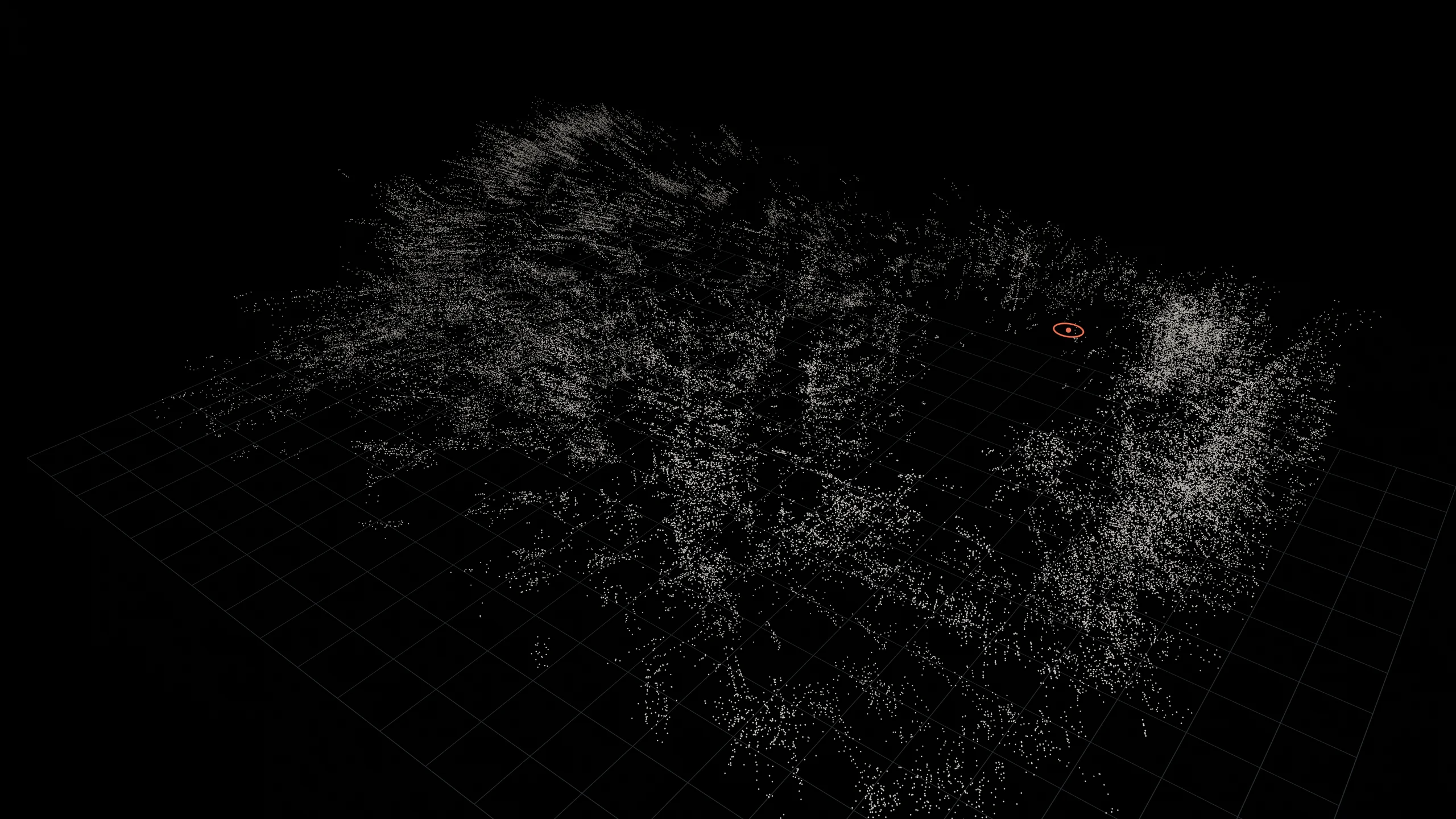
I set up two cameras on a humanoid robot so it could map a room in 3D and find itself in it.
The map the robot built
- From its two cameras, the robot built this 3D map of the lab: 62,112 points.
- When it sees these points again, it knows where it is.
Rendered in Blender from the map the robot saved, on a 1 m grid. The order the points appear in is illustrative.
The cameras
Measuring them
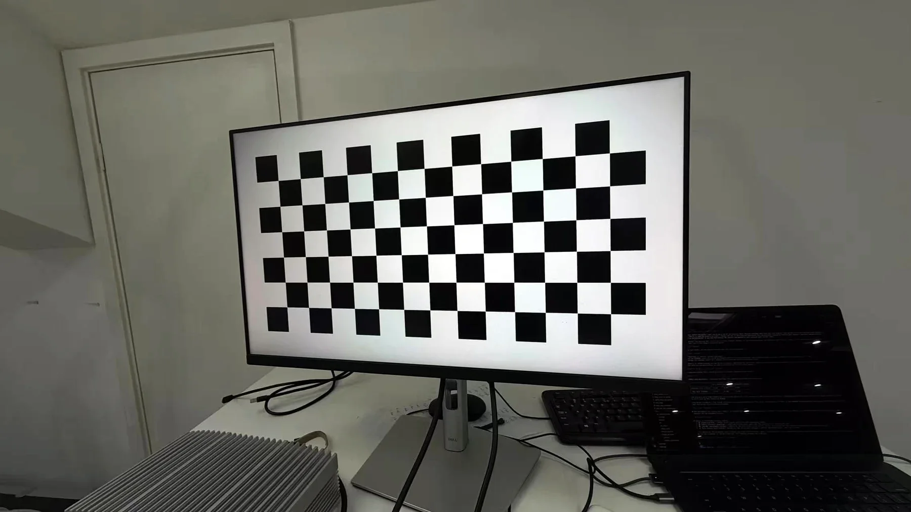
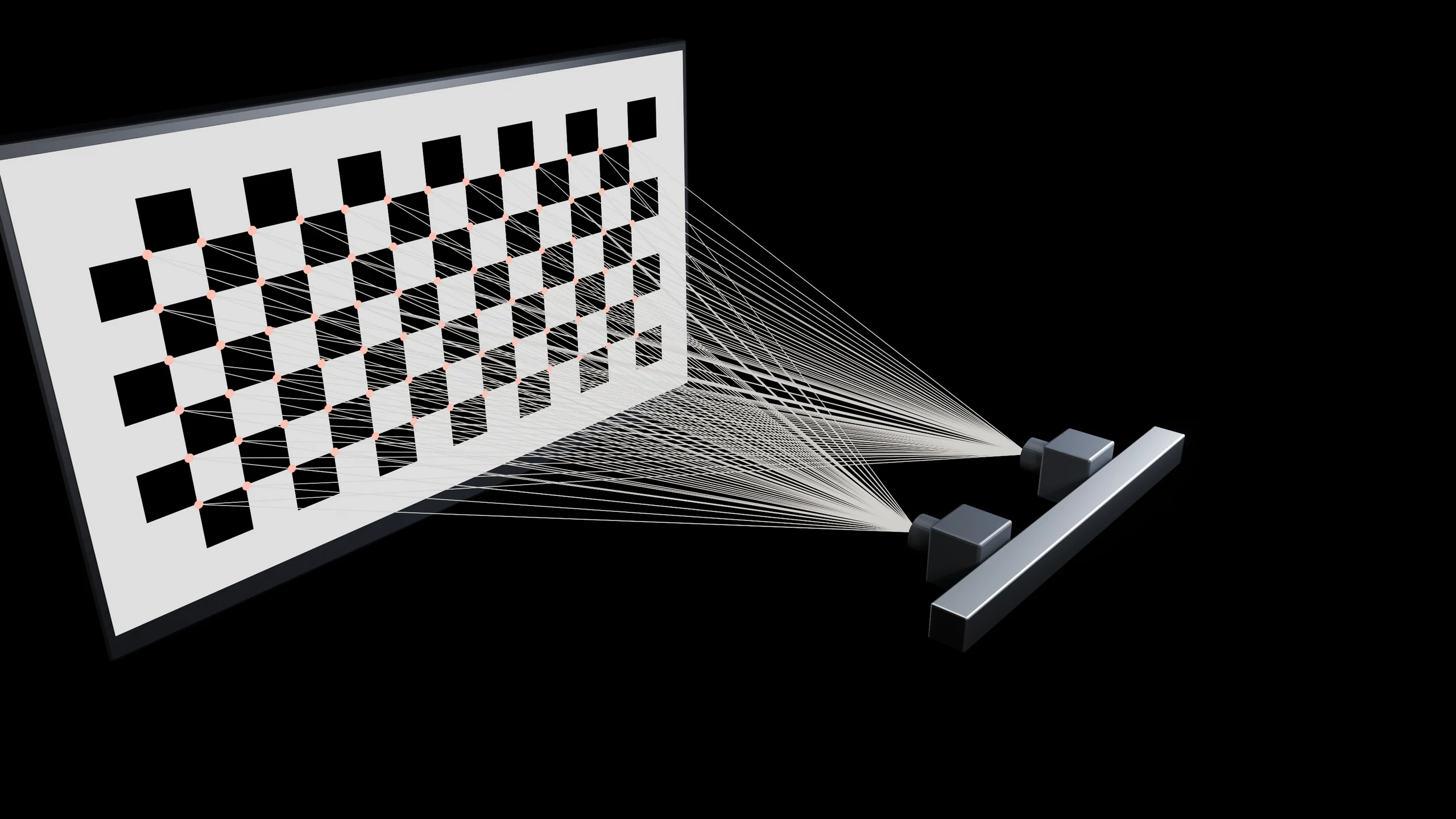
Measuring the cameras
- The robot’s two cameras, 12.4 cm apart, look at a checkerboard on a screen.
- Each corner is found in both cameras. Together, the lines measure the cameras exactly.
Rendered in Blender at real size. The camera bodies are simplified and the screen positions illustrative.
Average error after calibration
About a seventh of a pixel. The first attempt was off by 27 pixels, nearly 200 times as much.
One camera pixel, magnified. Cross: where a corner was seen. Ring: where the calibrated cameras put it.
Six rounds of calibration, from 27 pixels off to 0.137.
Timing
The robot’s motion sensor reads 100 times a second, but the readings arrived with uneven times. Its own clock made them exact.
A quarter second of motion readings, before and after.
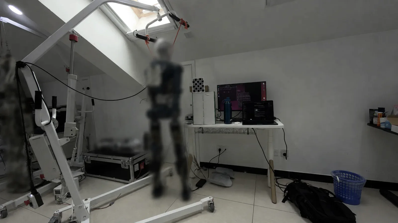
The robot hangs from ropes during testing, so I wrote a routine of bounces and turns to calibrate its motion sensor.
How much the position estimate wobbled while the robot stood still for a minute: four to six times less with the motion sensor.
On the robot
How far the robot’s position drifted in a minute standing still, to scale: 0.285 cm in the end, under the 1 cm goal.
Engineering notes for this chapter
The work started with RealSense feasibility tests on a workstation, moved to a four-wheel Jetson robot, and ended on a humanoid. Most of it was the system around the algorithm: stereo geometry, sensor timing, image quality, mapping modes, and tests that someone else could repeat.
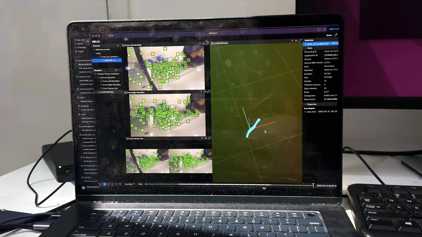
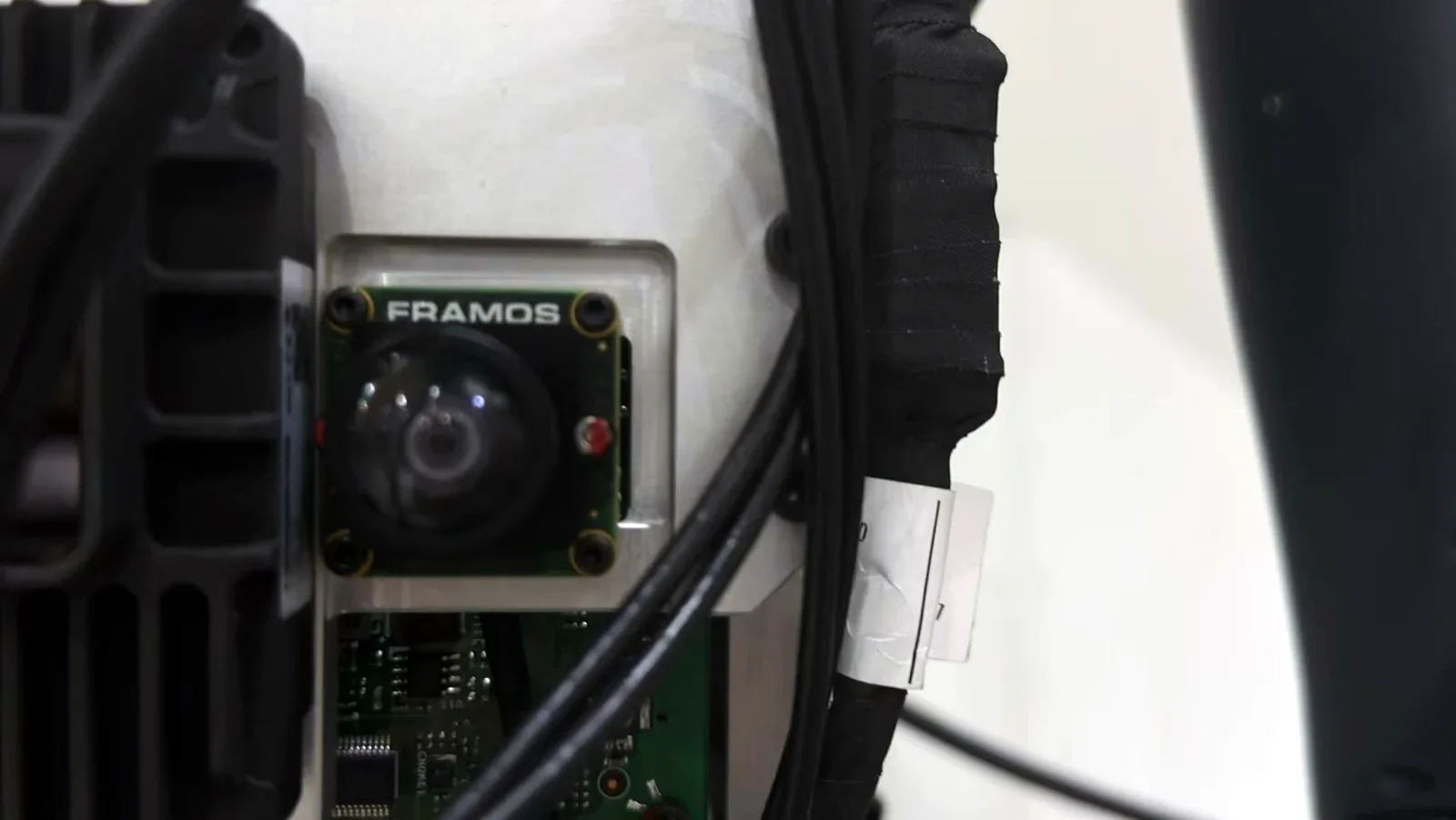
The robot carries FRAMOS stereo cameras built on Sony IMX900 sensors, an Xsens MTi-300 IMU and a Jetson. Before trusting any pose estimate I checked what the sensors were really delivering. The first finding was a driver default: an exposure setting of zero was being read as roughly 660 ms of exposure, which blurred every frame and slowed startup. A fixed 2 ms exposure raised the sharpness score from about 2.1 to 8.4.1
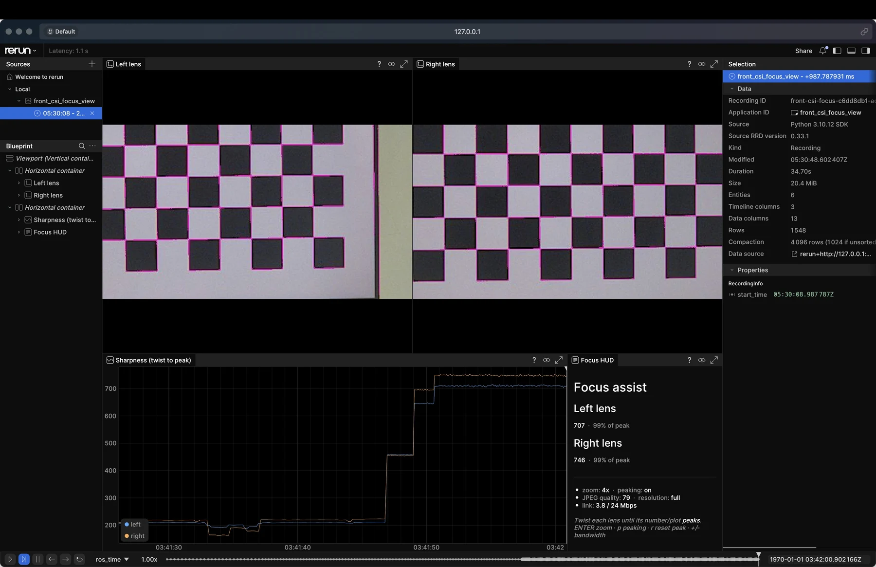
Two things limited calibration that no solver can fix: the camera’s own image processing, and focus you can’t see. The driver sharpened and denoised every frame by default. That looks better to a person, and it moves corner positions by fractions of a pixel. I turned both off, then built a focus mode in Rerun: a per-lens sharpness meter with edge peaking and a center zoom, measured on full-resolution crops so that a change in stream bandwidth never moves the reading.
For geometry I moved the target onto a Dell P2722H monitor. Its panel is 1920 by 1080 pixels, and the greatest common divisor of 1920 and 1080 is 120. So a board of 120-pixel squares tiles the screen with nothing left over and no rounding between squares.2 The board is 14 × 7 squares, which gives 13 × 6 inner corners, drawn by a small Electron tool I wrote. With OpenCV’s findChessboardCornersSB and its accuracy refinement, the stereo error fell from 27 px on the first solve to 0.137 px.
The last step was a solver setting. The standard pipeline blended the new camera intrinsics with older ones, 35% new, as a hedge from the days when the focal length wouldn’t hold still. By now the new values were the reliable ones, and blending pulled the focal length toward a stale number and raised the error to 0.342 px. Using the new intrinsics outright, which the log calls steer-1.0, gave 0.137.
A camera and an IMU can each be accurate and still disagree, because their clocks don’t match. The IMU’s messages were being stamped when they arrived at the computer, which put anywhere from 4.1 to 15.8 ms between samples that should have been exactly 10 ms apart. For calibration recordings I switched to the IMU’s hardware sample clock. Every interval then came out at 10.000 ms across 1,200 samples,3 and the camera–IMU alignment solved to a +2.0 ms offset with 80% inliers.
The robot hangs from two shoulder ropes and can’t move freely, so I wrote a 90-second excitation routine that produces linear acceleration anyway: vertical bounces into free fall and a catch, pitch and roll rocking through the lever arm, and fast reversals in yaw. A script checked the IMU statistics against pass and fail thresholds before any recording was accepted. With fusion on,4 the static jitter path fell from 63–75 cm to 11–18 cm.5
The robot also carries a RoboSense RS-E1 solid-state LiDAR, with a targetless LiDAR-to-camera calibration inherited from an earlier effort. Before comparing methods I fixed the cheapest real bug: the pipeline was still using stale camera intrinsics, with the principal point off by 54 pixels. Then I redid the calibration properly, using a 151-second slow-motion capture to fill in the sparse point cloud.
The answer was clear. Intensity-based targetless calibration can’t work on a sensor that never produces a dense, calibrated intensity image. By the criteria we had agreed on beforehand, I rolled the stack back to cuVSLAM with IMU fusion and wrote down why. ORB-SLAM3 kept running alongside as an open-source reference, so the final choice of platform rested on a comparison rather than a preference.
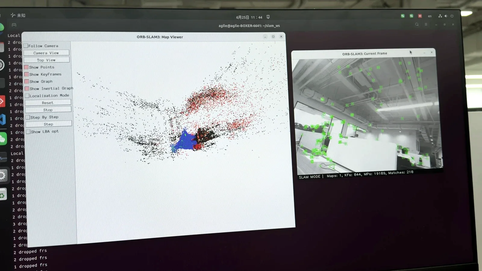
I packaged the stack into one-command mapping, localization and odometry modes, made saving the map part of shutdown, and versioned every calibration so the previous deployment is one command away. Intrinsics and camera–IMU extrinsics always ship together, because new intrinsics quietly invalidate the old extrinsics.
I left with a workflow as much as a result. It reproduces the calibration, flags a weak measurement early, and gets from a desk test to a running robot without hiding what is still uncertain. Most of what made the final number possible was staying with the problem through failed targets, timing jitter, image-quality limits and a change of platform.
| Stereo pairs detected | 1332 of 1332, none rejected |
|---|---|
| Camera–IMU alignment | 80% inliers (1399 of 1749), time offset +2.0 ms |
| IMU interval, calibration recordings | 10.000 ± 0.000 ms on the hardware clock |
| Static drift, 60 s | 0.285 cm at the end, 0.408 cm at peak, 0.07° of yaw |
| Live tracking | about 30 Hz on the Jetson |
- Sharpness here is the variance of the Laplacian, a standard blur measure. Higher is sharper.
- Squares of 24 mm would have needed 77.06 screen pixels each, so the grid lines would alternate between 77 and 78 pixels and bake a tenth of a pixel of error into the “ground truth.”
- At runtime the system keeps arrival timestamps, because the hardware clock’s anchor wanders against the computer’s clock over long runs.
- Fusion first trusted the IMU too much at its datasheet noise values and drifted 12–17 cm a minute. Telling the filter the IMU was seven times noisier stabilized it.
- Jitter path is the total distance the estimate wanders while the robot sits still, added up step by step. It measures high-frequency noise.
Revision history
| Rev | Stage | Where | What changed |
|---|---|---|---|
| A | System bring-up | cuVSLAM, FRAMOS stereo | Stereo SLAM, calibration and about 30 Hz real-time tracking running on the humanoid. |
| B | IMU refinement | Xsens MTi-300 | Timestamps and noise model corrected; fusion tuned and checked standing still and swinging. |
| C | Stereo recalibration | 9×6 screen board | Error down to 0.247 px; camera–IMU extrinsics re-run; first static drift under 1 cm. |
| D | Detector audit | findChessboardCornersSB | Every deployed calibration re-checked; stereo extrinsics cross-checked two ways. |
| E | Real auto-exposure | Argus AE | Sharp across lighting changes at runtime; fixed exposure kept for calibration capture. |
| F | Operator tools | Isaac ROS 3.2.6 | One-command slam_map, localize and odom modes; maps saved on shutdown. |
| G | Lens forensics | session 004 | A fingerprint on the left lens had more than doubled that camera’s error. Cleaned, the stereo error fell to 0.189 px. |
| H | LiDAR evaluation | RS-E1, FAST-LIVO2 | Targetless calibration shown unworkable on this sensor; rolled back on the evidence. |
| I | Unprocessed optics | Argus ISP, Rerun | Default sharpening and denoise turned off; focus mode with a per-lens sharpness meter. |
| J | Exact-scale target | Dell 13×6, steer-1.0 | 120-pixel squares, subpixel corner refinement; 0.137 px with no rejected pairs. |
| K | Coupled deployment | Jetson, on the robot | Intrinsics and realigned extrinsics shipped together; 0.285 cm over 60 s; one command to revert. |
Four seasons of competition
VEX since 2022, and FRC with Team 2584.
-
2022 8th grade
First build season
My first VEX season. No finished robot, but it stuck.
-
2023 9th grade
Finding a team
Builder and driver on a complete competition robot for the first time.
-
2024 10th grade
Starting a team
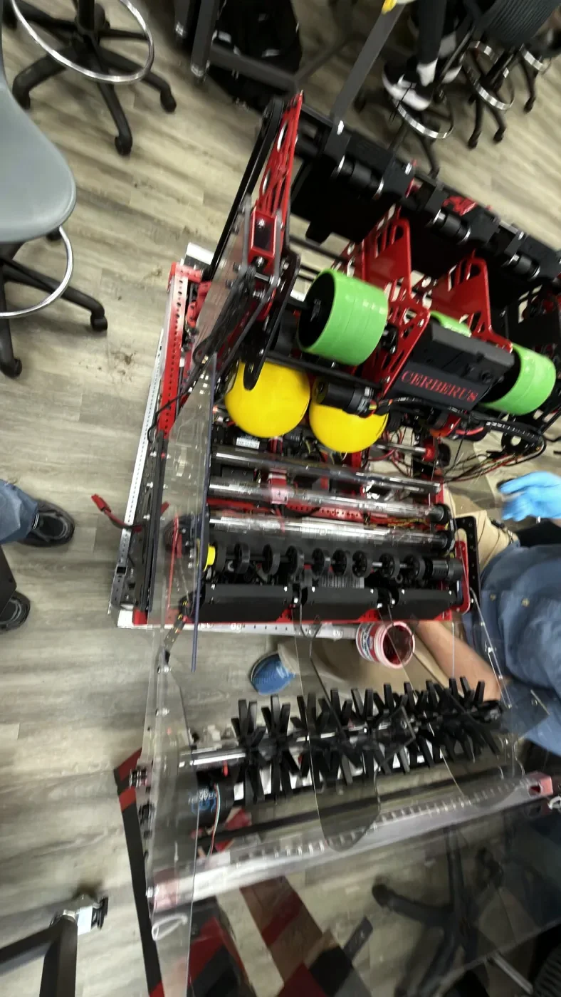
Started a five-person team and built on about two hours a day. Its intake was Cerberus.
-
2024–25 11th grade
Lead programmer
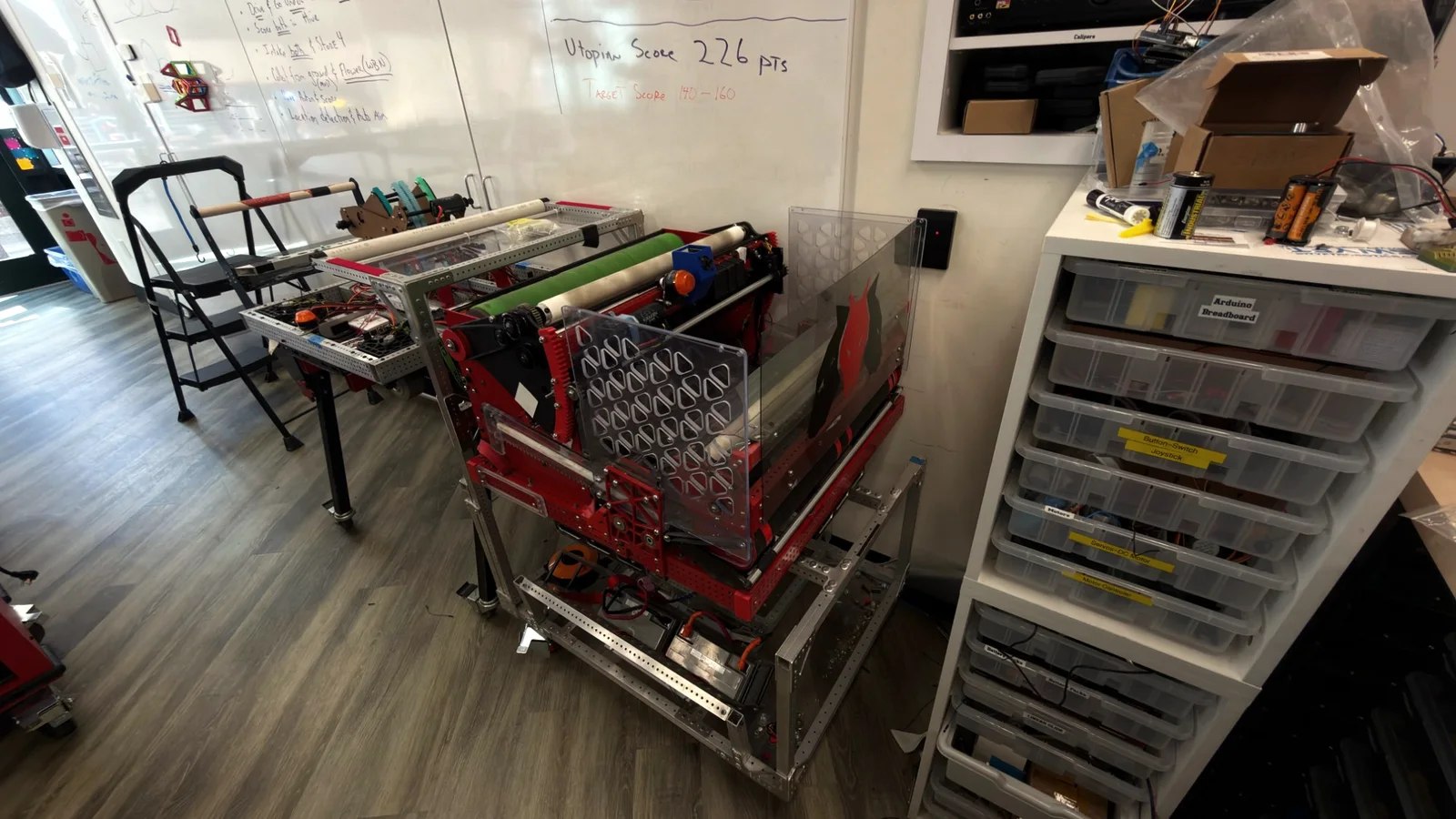
Rented a workspace and wrote the code that drives the robot on its own. The game was High Stakes.
FRC Team 2584
Programmer and parts-maker on a full-size FRC robot. I worked on its climb at the end of each match and on a turret that aims itself using a camera.
Record
- 2025VEX World Championship qualificationTeam 1658S
- 2025FRC Regional Championship qualificationTeam 2584
- 2024California State Championship qualificationOur new five-person team
- 2024USACO Gold DivisionCompetitive programming
About me
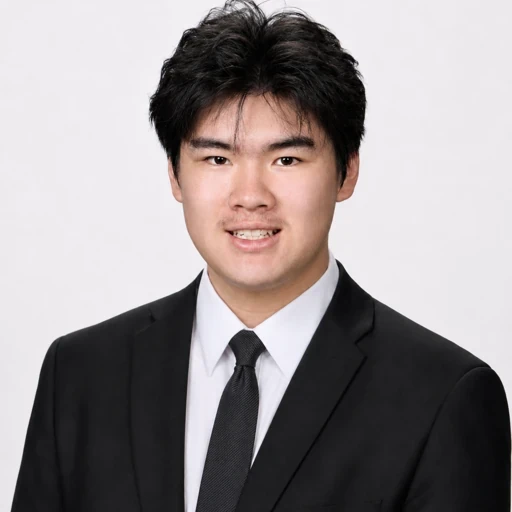
I’m a student at Viewpoint School. I design robot mechanisms, write the code that lets them drive themselves, and make the parts on CNC machines, laser cutters and 3D printers.
- Code
- C++, Python, Java
- Making
- CNC, laser cutting, 3D printing
- Design
- Onshape, Blender